Machine Learning

What libraries should I import?

pip install hmmlearn

pip install umap-learn

from hmmlearn import hmm
import umap
from sklearn.mixture import GaussianMixture
from sklearn import tree
from sklearn.tree import DecisionTreeClassifier
import pandas as pd
import numpy as np
import matplotlib.pyplot as plt

Recap

Dummy data for the following exercises is provided here.

file = '/Users/guillermo/Downloads/pose-3d.csv'
data = pd.read_csv(file, header=0)
coords = data.loc[:, ~data.columns.str.contains(
    'score|error|ncams|fnum|center|M_')]

Helper Functions

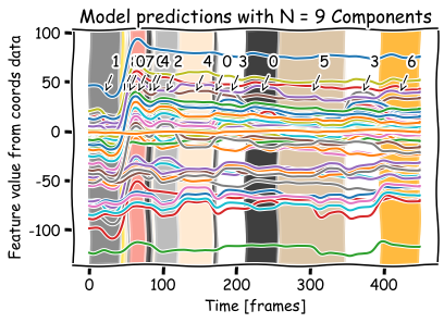
def plot_prediction(data, predictions):
    """
    This function will plot the time series data and mark the transitions between predicted classes.

    """
    colors = {"0": "black", "1": "dimgray", "2": "darkgray", "3": "white", "4": "bisque", "5": "tan", "6": "orange", "7": "salmon", "8": "gold", "9": "rosybrown", "10": "beige",
              "11": "thistle", "12": "peachpuff", "13": "khaki", "14": "skyblue", "15": "lightblue", "16": "lightsteelblue", "17": "lavender", "18": "mediumaquamarine", "19": "cadetblue"}
    n = max(predictions)+1
    name = [x for x in globals() if globals()[x] is data][0]
    yloc = max(np.max(data))-(max(np.max(data)) - min(np.min(data)))/8
    locy = yloc - (max(np.max(data)) - min(np.min(data)))/8
    with plt.xkcd():
        fig = plt.figure()
        ax = plt.axes()
        ax.plot(data)
        start_pred = 0
        for i in range(len(predictions)):
            if i == len(predictions)-1:
                end_pred = i+1
                ax.axvspan(start_pred, end_pred,
                           facecolor=colors["%d" % predictions[i]], alpha=0.5)
                loc = start_pred + (end_pred - start_pred)/2
                ax.annotate('%d' % predictions[i], xy=(loc, locy), xytext=(loc+10, yloc),
                            arrowprops=dict(arrowstyle="->", facecolor='black'))
            elif predictions[i] == predictions[i+1]:
                pass
            else:
                end_pred = i
                ax.axvspan(start_pred, end_pred,
                           facecolor=colors["%d" % predictions[i]], alpha=0.5)
                loc = start_pred + (end_pred - start_pred)/2
                ax.annotate('%d' % predictions[i], xy=(loc, locy), xytext=(loc+10, yloc),
                            arrowprops=dict(arrowstyle="->", facecolor='black'))
                start_pred = end_pred

        plt.xlabel("Time [frames]")
        plt.ylabel("Feature value from %s data" % name)
        plt.title('Model predictions with N = %d Components' % n)
        plt.show()
    return

Time segmentation with Hidden Markov Models

# Now we can train a Hidden markov Model with our coordinate data
model1 = hmm.GaussianHMM(n_components=9, covariance_type="full")
model1.fit(coords)

GaussianHMM(covariance_type='full', n_components=9)

hmm_pred = model1.predict(coords)

transition1 = model1.transmat_
transition1

array([[0.97619048, 0.        , 0.        , 0.        , 0.        ,
        0.        , 0.        , 0.02380952, 0.        ],
       [0.        , 0.93442623, 0.01639344, 0.01639344, 0.01639344,
        0.        , 0.        , 0.        , 0.01639344],
       [0.        , 0.        , 0.97222222, 0.        , 0.        ,
        0.        , 0.02777778, 0.        , 0.        ],
       [0.        , 0.01234568, 0.        , 0.97530864, 0.        ,
        0.01234568, 0.        , 0.        , 0.        ],
       [0.        , 0.        , 0.        , 0.01111111, 0.98888889,
        0.        , 0.        , 0.        , 0.        ],
       [0.        , 0.        , 0.        , 0.        , 0.        ,
        1.        , 0.        , 0.        , 0.        ],
       [0.        , 0.0212766 , 0.        , 0.        , 0.        ,
        0.        , 0.9787234 , 0.        , 0.        ],
       [0.        , 0.09090909, 0.        , 0.        , 0.        ,
        0.        , 0.        , 0.90909091, 0.        ],
       [0.        , 0.03846154, 0.        , 0.        , 0.        ,
        0.        , 0.        , 0.        , 0.96153846]])

plot_prediction(coords, hmm_pred)

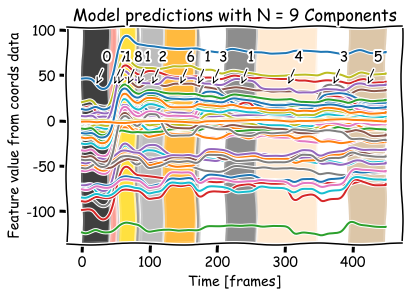
Gaussian Mixture Model

gmm_pred = GaussianMixture(
    n_components=9, covariance_type='full').fit_predict(coords)

plot_prediction(coords, gmm_pred)

Decision Trees

dtree = DecisionTreeClassifier()
dtree = dtree.fit(coords, hmm_pred)

plt.figure(figsize=(30, 20))
tree.plot_tree(dtree, feature_names=coords.columns, fontsize=12)
plt.show()

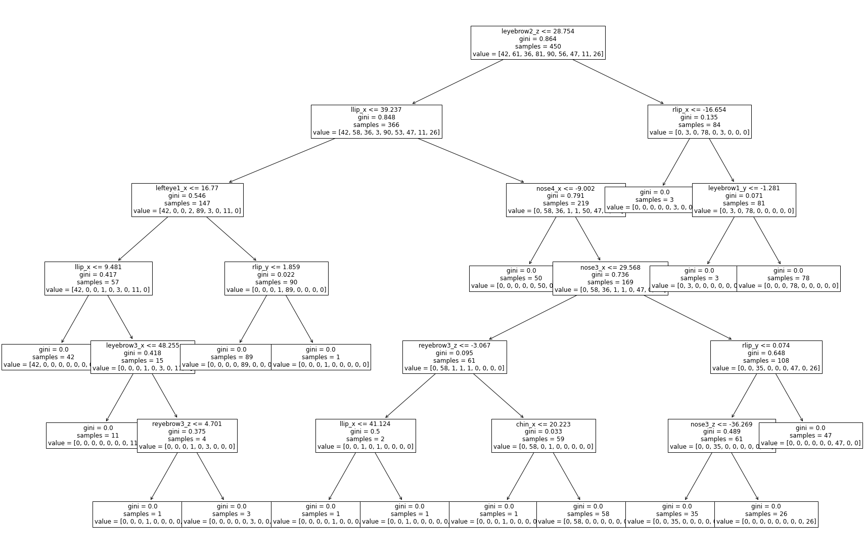
n = 100
print(
    f'Prediction from decision tree for frame {n}: {dtree.predict(coords[n:n+1])}')

Prediction from decision tree for frame 100: [2]

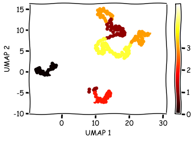
UMAP dimensionality reduction

mapper = umap.UMAP(metric='euclidean', n_neighbors=30, min_dist=0.99,
                   random_state=42, init='random').fit_transform(coords)
print(f"Umap data ready with shape {np.shape(mapper)}")

OMP: Info #271: omp_set_nested routine deprecated, please use omp_set_max_active_levels instead.

Umap data ready with shape (450, 2)

umap1 = mapper[:, 0]
umap2 = mapper[:, 1]
labels = hmm_pred

with plt.xkcd():
    plt.figure()
    cmap = plt.cm.get_cmap('hot')
    plt.scatter(umap1, umap2, c=labels.astype(np.float64), cmap=cmap)
    plt.xlabel('UMAP 1')
    plt.ylabel('UMAP 2')
    plt.colorbar(ticks=range(4))
    plt.clim(0, 5)
    plt.show()